시계열 데이터를 이미지로 바꿔보자!

이번에는 시계열 데이터를 이미지로 변환하는 방법에 대해서 알아보자!

pyts는 시계열 분류, 클러스터링 및 전처리를 위한 Python 라이브러리이다. 시계열 데이터 작업을 위한 다양한 메서드를 지원한다! 여기서 제공하는 기능 중 하나인 시계열 이미지 변환 기능을 사용해보겠다.

총 3가지 방법을 지원한다. 그럼 하나하나씩 살펴보자

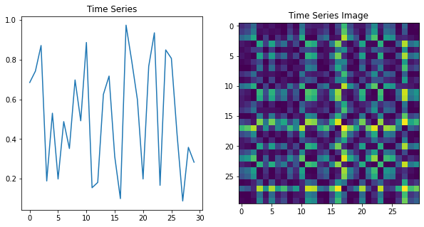
Gramian Angular Field(GAF)

GAF의 기본 아이디어는 시계열의 포인트 쌍 간의 시간적 상관 관계를 2D 이미지로 매핑한것이다.
이 작업은 시계열의 내적을 나타내는 Gramian 행렬을 구성하여 수행된다.
Gramian행렬은 SVD((Singular Value Decomposition)를 계산하여 이미지 표현으로 변환된다.

import numpy as np
import matplotlib.pyplot as plt
from mpl_toolkits.axes_grid1 import ImageGrid
from pyts.image import GramianAngularField, MarkovTransitionField, RecurrencePlot

# 랜덤 시계열데이터 생성
rng = np.random.default_rng()
time_series = rng.random((50, 30))
print(f"시계열 데이터: {time_series.shape}")

# 모델 생성
transformer = GramianAngularField()

# 시계열 데이터를 이미지로 변경
images = transformer.fit_transform(time_series)
print(f"이미지: {images.shape}")

# 시각화
plt.figure(figsize=(10, 5))
plt.subplot(121)
plt.plot(time_series[0])
plt.title("Time Series")

plt.subplot(122)
plt.imshow(images[0])
plt.title("Time Series Image")

plt.show()

시계열 데이터: (50, 30)
이미지: (50, 30, 30)

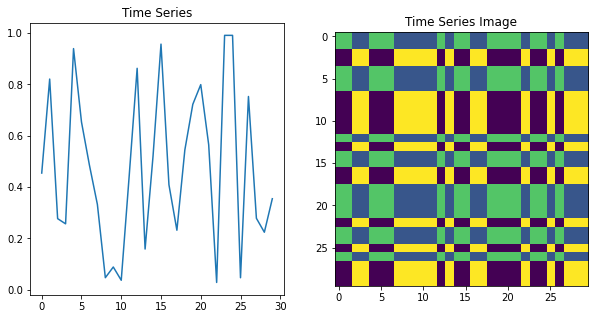
Markov Transition Fields(MTF)

MTF의 기본 아이디어는 시계열의 연속 지점 사이의 전환 확률을 캡처하는 것이다.
시계열은 겹치는 창으로 나뉘고 각 창에 대해 창의 지점 간 전환 확률을 나타내는 행렬이 구성된다. 그런 다음 이러한 행렬을 연결하여 시계열의 2D 이미지 표현을 형성한다.
결과 이미지는 원본 데이터의 시계열간의 순차적 관계를 캡처하는 시계열을 나타낸다.

# 랜덤 시계열데이터 생성
rng = np.random.default_rng()
time_series = rng.random((50, 30))
print(f"시계열 데이터: {time_series.shape}")

# 모델 생성
transformer = MarkovTransitionField(n_bins=2)

# 시계열 데이터를 이미지로 변경
images = transformer.fit_transform(time_series)
print(f"이미지: {images.shape}")

# 시각화
plt.figure(figsize=(10, 5))
plt.subplot(121)
plt.plot(time_series[0])
plt.title("Time Series")

plt.subplot(122)
plt.imshow(images[0])
plt.title("Time Series Image")

plt.show()

시계열 데이터: (50, 30)
이미지: (50, 30, 30)

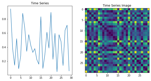
Recurrence Plot(RP)

RP는 시계열의 반복 패턴을 그래픽으로 표현한 것이다. 비선형 역학 분야에서 널리 사용된다.
RP의 기본 아이디어는 시계열의 각 지점을 다른 모든 지점과 비교하고 그 사이의 거리가 지정된 임계값보다 작은지 확인한다.
두 점 사이의 거리가 임계값보다 작으면 RP의 해당 위치에 점이 그려진다.
결과 이미지는 시계열의 반복 패턴을 보여주는 이진 행렬로 보여진다.
RP는 주기적인 동작 및 추세와 같은 시계열의 다양한 기능을 식별하는데 사용할 수 있다.

# 랜덤 시계열데이터 생성
rng = np.random.default_rng()
time_series = rng.random((50, 30))
print(f"시계열 데이터: {time_series.shape}")

# 모델 생성
transformer = RecurrencePlot()

# 시계열 데이터를 이미지로 변경
images = transformer.fit_transform(time_series)
print(f"이미지: {images.shape}")

# 시각화
plt.figure(figsize=(10, 5))
plt.subplot(121)
plt.plot(time_series[0])
plt.title("Time Series")

plt.subplot(122)
plt.imshow(images[0])
plt.title("Time Series Image")

plt.show()

시계열 데이터: (50, 30)
이미지: (50, 30, 30)

참고자료

• pyts문서