
오토인코더를 이용한 이상탐지(Anomaly Detection with AutoEncoder)
본 예제는 기본적으로 텐서플로우 공식 사이트 예제를 이용하고 추가로 코드를 작성하였습니다!
이상탐지(Anomaly Detection이란?)
정상 비정상 문제를 구별해내는 문제이다. 쉽게 말해 정상인 데이터와 비정상인 데이터를 구분하는 작업이라고 생각하면 된다. 이상탐지는 label 유무에 따라 세가지로 나뉜다
- Supervised Anomaly Detection
주어진 학습 데이터 셋에 정상과 비정상의 Data와 Label이 모두 존재하는 경우이다. 지도학습 방식이기 때문에 다른 방법 대비 정확도가 높은 특징이 있다. - Semi-supervised Anomaly Detection
Supervised Anomaly Detection의 가장 큰 문제는 데이터 불균형 문제이다. 실제로 비정상 데이터를 확보하는데 많은 시간과 비용이 들어간다. 이 방식은 정상 데이터만 이용해서 모델을 학습하는 방식이다. - Unsupervised Anomaly Detection
정상 데이터도 Labeling이 힘들거나 부족할 것을 대비해 대부분의 데이터가 정상 데이터라고 가정하고 Label없이 학습을 시키는 방법이다.
코드
# 필요한 모듈 Imoport
import matplotlib.pyplot as plt
import numpy as np
import pandas as pd
import tensorflow as tf

from sklearn.metrics import accuracy_score, precision_score, recall_score
from sklearn import metrics
import seaborn as sns
from sklearn.model_selection import train_test_split
from tensorflow.keras import layers, losses
from tensorflow.keras.models import Model
# 데이터셋 로드
dataframe = pd.read_csv('http://storage.googleapis.com/download.tensorflow.org/data/ecg.csv', header=None)
raw_data = dataframe.values
dataframe.head()
| 0 | 1 | 2 | ... | 138 | 139 | 140 | |
|---|---|---|---|---|---|---|---|
| 0 | -0.112522 | -2.827204 | -3.773897 | ... | 0.925286 | 0.193137 | 1.0 |
| 1 | -1.100878 | -3.996840 | -4.285843 | ... | 1.119621 | -1.436250 | 1.0 |
| 2 | -0.567088 | -2.593450 | -3.874230 | ... | 0.904227 | -0.421797 | 1.0 |
| 3 | 0.490473 | -1.914407 | -3.616364 | ... | 1.403011 | -0.383564 | 1.0 |
| 4 | 0.800232 | -0.874252 | -2.384761 | ... | 1.614392 | 1.421456 | 1.0 |
5 rows × 141 columns
텐서플로우에서 제공하는 ECG데이터. 0은 비정상, 1은 정상 데이터임. 이번 예제에서는 정상과 비정상 데이터 모두 Labeling이 되어 있는 상태이기 때문에 Supervised Anomaly Detection이라고 할 수 있다.
# 140번째 column은 라벨임
labels = raw_data[:, -1]

# 마지막 column을 제외하고는 모두 data임
data = raw_data[:, 0:-1]

# train, test 분할
train_data, test_data, train_labels, test_labels = train_test_split(
    data, labels, test_size=0.2, random_state=21)
# 데이터 정규화
min_val = tf.reduce_min(train_data)
max_val = tf.reduce_max(train_data)

train_data = (train_data - min_val) / (max_val - min_val)
test_data = (test_data - min_val) / (max_val - min_val)

train_data = tf.cast(train_data, tf.float32)
test_data = tf.cast(test_data, tf.float32)
# 라벨을 boolean으로 타입 변경(0은 False(비정상), 1은 True(정상)))
train_labels = train_labels.astype(bool)
test_labels = test_labels.astype(bool)

# 정상 데이터
normal_train_data = train_data[train_labels]
normal_test_data = test_data[test_labels]

# 비정상 데이터
anomalous_train_data = train_data[~train_labels]
anomalous_test_data = test_data[~test_labels]
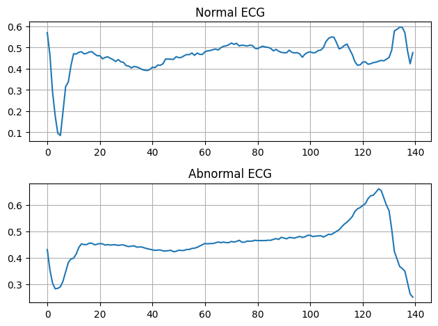
# 정상, 비정상 데이터 시각화
plt.subplot(2, 1, 1)
plt.plot(np.arange(140), normal_train_data[0])
plt.title("Normal ECG")
plt.grid()

plt.subplot(2, 1, 2)
plt.plot(np.arange(140), anomalous_train_data[0])
plt.title("Abnormal ECG")
plt.grid()

plt.tight_layout()
plt.show()
# Autoencoder모델 정의
class AnomalyDetector(Model):
    def __init__(self):
        super(AnomalyDetector, self).__init__()
        self.encoder = tf.keras.Sequential([
            layers.Dense(32, activation="relu"),
            layers.Dense(16, activation="relu"),
            layers.Dense(8, activation="relu")])

        self.decoder = tf.keras.Sequential([
            layers.Dense(16, activation="relu"),
            layers.Dense(32, activation="relu"),
            layers.Dense(140, activation="sigmoid")])

    def call(self, x):
        encoded = self.encoder(x)
        decoded = self.decoder(encoded)
        return decoded

autoencoder = AnomalyDetector()
autoencoder.compile(optimizer='adam', loss='mae')
# 정상 데이터로만 훈련
history = autoencoder.fit(normal_train_data, normal_train_data,
          epochs=20,
          batch_size=512,
          validation_data=(test_data, test_data))
Epoch 1/20
5/5 [==============================] - 1s 45ms/step - loss: 0.0575 - val_loss: 0.0530
Epoch 5/20
5/5 [==============================] - 0s 10ms/step - loss: 0.0444 - val_loss: 0.0451
Epoch 10/20
5/5 [==============================] - 0s 9ms/step - loss: 0.0293 - val_loss: 0.0385
Epoch 15/20
5/5 [==============================] - 0s 17ms/step - loss: 0.0237 - val_loss: 0.0349
Epoch 20/20
5/5 [==============================] - 0s 9ms/step - loss: 0.0210 - val_loss: 0.0328
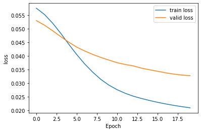
정상데이터로만 훈련하는 이유는 모델 훈련이 끝난 후 reconstruction작업을 하는데, 정상 데이터로만 훈련을 해서 정상과 비정상 데이터에 대한 reconstruction error를 비교해야 하기 때문임. 반면 test data는 정상+비정상이 같이 있음
# 훈련결과 시각화
plt.plot(history.history['loss'], label='train loss')
plt.plot(history.history['val_loss'], label='valid loss')
plt.legend()
plt.xlabel('Epoch'); plt.ylabel('loss')
plt.show()
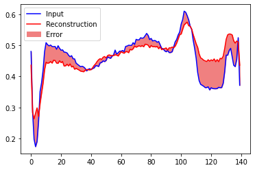
# 정상데이터 재구성결과
encoded_imgs = autoencoder.encoder(normal_test_data).numpy()
decoded_imgs = autoencoder.decoder(encoded_imgs).numpy()

plt.plot(normal_test_data[0], 'b')
plt.plot(decoded_imgs[0], 'r')
plt.fill_between(np.arange(140), decoded_imgs[0], normal_test_data[0], color='lightcoral')
plt.legend(labels=["Input", "Reconstruction", "Error"])
plt.show()
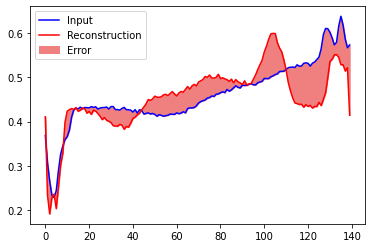
# 비정상데이터 재구성결과
encoded_imgs = autoencoder.encoder(anomalous_test_data).numpy()
decoded_imgs = autoencoder.decoder(encoded_imgs).numpy()

plt.plot(anomalous_test_data[0], 'b')
plt.plot(decoded_imgs[0], 'r')
plt.fill_between(np.arange(140), decoded_imgs[0], anomalous_test_data[0], color='lightcoral')
plt.legend(labels=["Input", "Reconstruction", "Error"])
plt.show()
# 재구성 결과와 train data(정상만)의 loss를 구함
reconstructions = autoencoder.predict(normal_train_data)
train_loss = tf.keras.losses.mae(reconstructions, normal_train_data)
74/74 [==============================] - 0s 1ms/step
# 재구성 오류를 이용해서 threshold설정
threshold = np.mean(train_loss) + np.std(train_loss)
print("Threshold: ", threshold)
Threshold: 0.032247376 > 이 threshold 이상의 값은 다 비정상으로 간주함.
# test data로 loss를 구함.
reconstructions = autoencoder.predict(test_data)
test_loss = tf.keras.losses.mae(reconstructions, test_data)
32/32 [==============================] - 0s 1ms/step
test_loss의 실제 값을 출력해보면 대부분 0.03 이상이다.
# 정상 비정상 데이터 시각화
error_df = pd.DataFrame({'Reconstruction_error': test_loss,
                         'True_class': test_labels.tolist()})

groups = error_df.groupby('True_class')
fig, ax = plt.subplots()

for name, group in groups:
    ax.plot(group.index, group.Reconstruction_error, marker='o', ms=3.5, linestyle='',
            label= "Break" if name == 1 else "Normal")
ax.hlines(threshold, ax.get_xlim()[0], ax.get_xlim()[1], colors="r", zorder=100, label='Threshold')
ax.legend()
plt.title("Reconstruction error for different classes")
plt.ylabel("Reconstruction error")
plt.xlabel("Data point index")
plt.show()
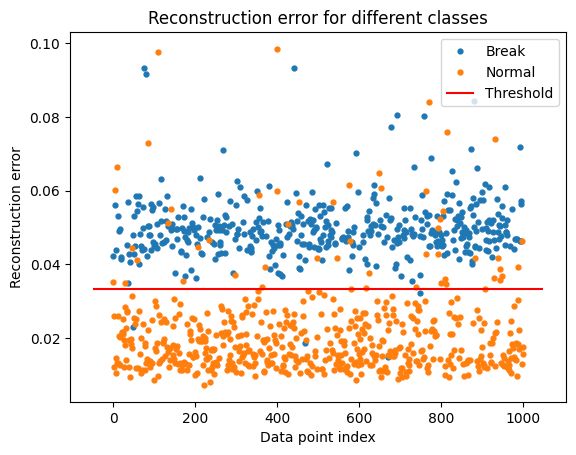
임계값을 기준으로 비정상 데이터는 값이 큰 것을 알수있다.
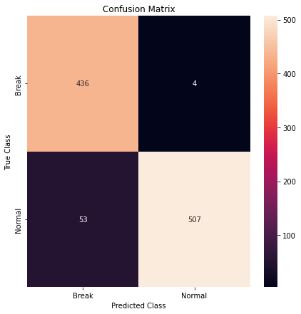
# 히트맵 시각화
LABELS = ['Break', 'Normal']
pred_y = [0 if e > threshold else 1 for e in error_df['Reconstruction_error'].values]
conf_matrix = metrics.confusion_matrix(error_df['True_class'], pred_y)
plt.figure(figsize=(7, 7))
sns.heatmap(conf_matrix, xticklabels=LABELS, yticklabels=LABELS, annot=True, fmt='d')
plt.title('Confusion Matrix')
plt.xlabel('Predicted Class'); plt.ylabel('True Class')
plt.show()
y_test = test_labels.astype('int')
# score 출력
print(accuracy_score(y_test, pred_y))
print(recall_score(y_test, pred_y))
print(precision_score(y_test, pred_y))
print(f1_score(y_test, pred_y))
0.943
0.9053571428571429
0.9921722113502935
0.9467787114845939
참고 자료
오늘의 정리
- 정상 데이터만으로 학습 시키는 이유는 정상 reconstruction error와 비정상 reconstruction error를 비교하기 위함
- Basic AE모델인데도 꽤 정확하게 탐지를 하는 것을 알 수 있다!!
댓글남기기