딥러닝 순전파

순전파(Foward propagation)란?

신경망모델의 입력층부터 출력층까지 순서대로 변수들을 계산하여 최종 출력으로 나오는 것.
각 은닉층에는 활성화함수(sigmoid, tanh, relu)등을 사용한다.

import numpy as np

# sigmoid 함수 정의
def sigmoid(x):
    return 1 / (1 + np.exp(-x))

# 기울기를 구하기 위한 수치미분 함수 정의
def numerical_gradient(f, x):
    h = 1e-4 # 0.0001
    grad = np.zeros_like(x)
    
    it = np.nditer(x, flags=['multi_index'], op_flags=['readwrite'])
    while not it.finished:
        idx = it.multi_index
        tmp_val = x[idx]
        x[idx] = tmp_val + h
        fxh1 = f(x) # f(x+h)
        
        x[idx] = tmp_val - h 
        fxh2 = f(x) # f(x-h)
        grad[idx] = (fxh1 - fxh2) / (2*h)
        
        x[idx] = tmp_val
        it.iternext()   
        
    return grad

# MSE Loss 정의
def MSE(y, t):
    return ((y-t)**2).mean(axis=None)

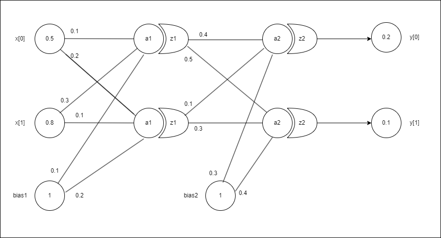
예제로 사용하는 신경망의 구조

# input 값
input_value = np.array([0.5, 0.8])
# 실제 값(원하는 값)
true_value = np.array([0.2, 0.1])
# 1층 가중치
weight1 = np.array([[0.1, 0.2],[0.3, 0.1]])
# 1층 편향
bias1 = np.array([0.1, 0.2])
# 2층 가중치
weight2 = np.array([[0.4, 0.5],[0.1, 0.3]])
# 2층 편향
bias2 = np.array([0.3, 0.4])

class Test():
    def __init__(self):
        pass
    # input_value와 각 층의 가중치와 편향의 곱 연산한 값을 출력
    def predict(self, x):
        a1 = np.dot(x, weight1) + bias1
        z1 = sigmoid(a1)
        a2 = np.dot(z1, weight2) + bias2
        y = sigmoid(a2)
        return y
    
    # input_value와 true_value의 차이를 계산
    def loss(self, x, t):
        y = self.predict(x)
        return MSE(y, t)
        
    # loss값과 각 층의 가중치와 편향의 기울기를 구함
    def grad_func(self, x, t):

        loss_W = lambda W: self.loss(x, t)
        
        grads_weight1 = numerical_gradient(loss_W, weight1)
        grads_weight2 = numerical_gradient(loss_W, weight2)
        grads_bias1 = numerical_gradient(loss_W, bias1)
        grads_bias2 = numerical_gradient(loss_W, bias2)
        
        return grads_weight1, grads_weight2, grads_bias1, grads_bias2

network = Test()
weight1_list = []
weight2_list = []
bias1_list = []
bias2_list = []
grad_list = []
for i in range(3000):
    grad = network.grad_func(input_value, true_value)
    # 가중치 수정
    weight1 -= 0.1 * grad[0]    # 이 부분은 경사 하강법(0.1은 learning rate라고 하고 임의로 설정 가능하다.)
    weight2 -= 0.1 * grad[1]    # (기존 매개변수 - 기울기*learing rate)로 가중치를 조금씩 수정한다.
    bias1 -= 0.1 * grad[2]      # 여기서는 3000번 반복하여 기울기를 점차 줄인다
    bias2 -= 0.1 * grad[3]      # 즉, 기울기가 최소(0)에 가까워 질 때까지 기울기를 줄이고 가중치를 저장
    new_predict = network.predict(input_value)
    new_loss = MSE(new_predict, true_value)
    # 가중치, 편향, 기울기 저장
    weight1_list.append(weight1)
    weight2_list.append(weight2)
    bias1_list.append(bias1)
    bias2_list.append(bias2)
    grad_list.append(grad)
    if i % 150 == 0:
        print(f"[{i}] 예측: {new_predict}, 손실: {new_loss}")

경사법으로 학습을 시작

[0] 예측: [0.64106615 0.70142718], 손실: 0.27812700471578844
[150] 예측: [0.30649078 0.26057261], 손실: 0.018561924206582828
[300] 예측: [0.238731   0.17752054], 손실: 0.0037547623725053135
[450] 예측: [0.21658743 0.14735127], 손실: 0.0012586428306008053
[600] 예측: [0.20747413 0.13194776], 손실: 0.0005382610348171978
[750] 예측: [0.20337815 0.12273718], 손실: 0.0002641956167999194
[900] 예측: [0.20147892 0.11671756], 손실: 0.00014083198842101307
[1050] 예측: [0.20059636 0.11255778], 손실: 7.902677864841668e-05
[1200] 예측: [0.2001941 0.1095738], 손실: 4.5847693122934905e-05
[1350] 예측: [0.20001903 0.1073766 ], 손실: 2.7207278543627808e-05
[1500] 예측: [0.19995006 0.10572796], 손실: 1.6406009640097618e-05
[1650] 예측: [0.19992923 0.10447365], 손실: 1.0009270002713057e-05
[1800] 예측: [0.19992906 0.10350938], 손실: 6.1603911651294744e-06
[1950] 예측: [0.19993677 0.10276222], 손실: 3.8169319263361906e-06
[2100] 예측: [0.1999466  0.10217978], 손실: 2.377149733919919e-06
[2250] 예측: [0.19995616 0.10172363], 손실: 1.486403770528686e-06
[2400] 예측: [0.19996455 0.10136508], 손실: 9.323438739013135e-07
[2550] 예측: [0.19997157 0.10108245], 손실: 5.862497258460017e-07
[2700] 예측: [0.19997731 0.10085917], 손실: 3.693430078741367e-07
[2850] 예측: [0.19998193 0.10068247], 손실: 2.330456372621908e-07

150번마다 예측값과 손실값을 출력해보았더니 예측값은 우리가 설정했던 true_value의 값과 거의 같고 손실은 점점 줄어드는 것을 볼 수 있다.

print(grad_list[0])
print(grad_list[1])

    grad_list[0]
    (array([[0.01247645, 0.00577953], [0.01996232, 0.00924725]]), 
    array([[0.06076802, 0.0750013 ], [0.06052245, 0.07469821]]), 
    array([0.0249529 , 0.01155907]), 
    array([0.10191142, 0.12578144]))

    grad_list[1]
    (array([[0.01228974, 0.00559548], [0.01966358, 0.00895277]]), 
    array([[0.06040114, 0.07496181], [0.06021838, 0.07473499]]), 
    array([0.02457948, 0.01119096]), 
    array([0.10148947, 0.12595514]))

기울기를 출력해보면 아주 미세하지만 갈수록 0으로 가까워 지고 있다.

def predict(x):
    a1 = np.dot(x, weight1_list[-1]) + bias1_list[-1]
    z1 = sigmoid(a1)
    a2 = np.dot(z1, weight2_list[-1]) + bias2_list[-1]
    y = sigmoid(a2)
    return y

predict(input_value)

array([0.19998561, 0.10054327])

학습을 해서 나온 가중치와 편향으로 예측을 하면 같은 추론을 한다. 다른말로, 적절한 가중치와 편향을 알면 굳이 학습이 필요없다는 얘기(하지만 현실은 적절한 가중치와 편향을 알 수가 없다…)

오늘의 정리

1. 딥러닝에서의 학습이란 적절한 가중치와 편향을 찾는 과정임.
2. 적절한 매개변수는 경사하강법을 통해서 구함

참고자료

• 밑바닥부터 시작하는 딥러닝